
Direct Field Coverage – Where intuition and modeling meet
This is a short case-study to illustrate the role of computer modeling when placing loudspeakers in a venue. Why guess when you can get it right?
Coverage is not intuitive. If you get it wrong, there’s no way to fix it with equalization. Since it is math, there’s no need to guess. Calculating the direct field coverage from measured loudspeaker balloon data is perhaps the most accurate aspect of sound system computer modeling.
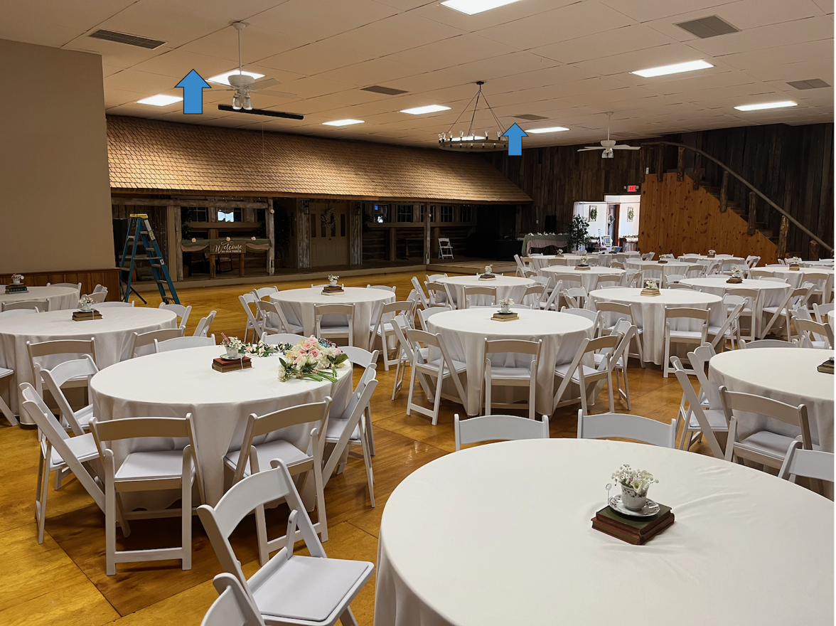 Photo 1 – The event venue with proposed loudspeaker placements (blue arrows).
There’s a Room Like This Near You
A local events venue was having some major sound problems during their events. The complaints included the usual stuff – muffled sound, feedback, and uneven coverage. Two “speaker on sticks” are setup for each event. These are typical 112H internally-powered units (a 12″ low frequency loudspeaker + high frequency horn). Photo 1 was taken from the back row.
Figure 1 shows a direct field map for the typical placement and aiming. The loudspeakers are just above ear height. The system is mono, and the objective is to cover the audience plane evenly. With this setup, the level delta over the audience plane is about 15 dB. How do we reduce it?
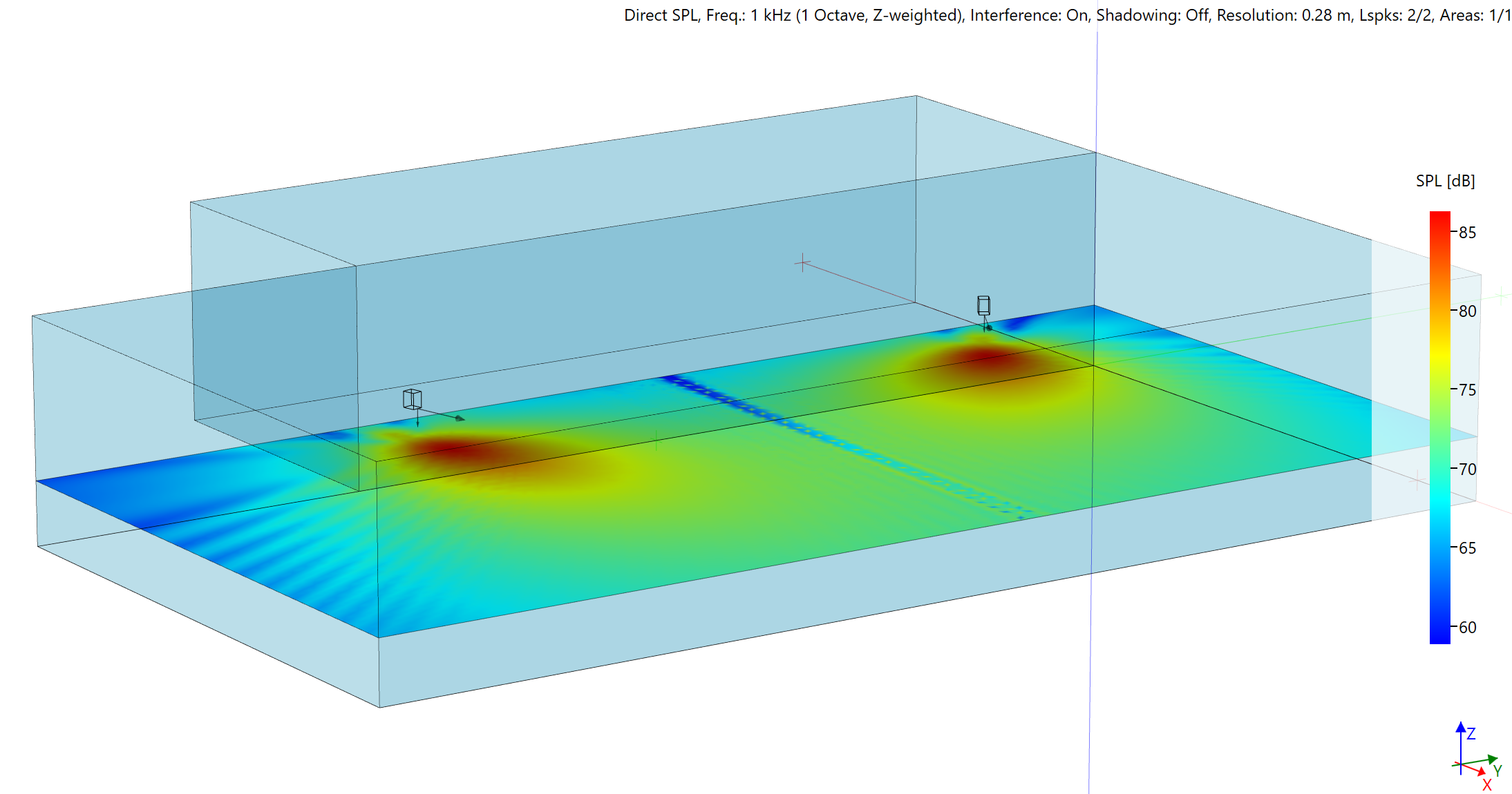
Figure 1 – The direct field coverage with loudspeakers on floor stands (EASE 5®).
Reposition the Loudspeakers
I suggested that the loudspeakers be flown. This would make them more equidistant from all listeners, thus evening out the coverage. This “overhead-zoned, distributed” approach would not require a loudspeaker model change.
Some things that must be considered:
1. Is the ceiling high enough to allow even coverage front-to-back?
2. Would two units be enough, or should another one be added?
3. Is the achievable SPL high enough?
These are questions that can be addressed by intuition, but it only takes a few minutes to model the space. The room is acoustically “live” but there is no budget for treatment. Only the audience planes are needed for direct field coverage, but I added the walls and ceiling to provide a visual reference for placing the loudspeakers.
Loudspeaker Data
The loudspeaker is a popular make and model, and a GLL data file is available from the manufacturer. After reviewing it I decided to measure my own. This required the following measurements:
1. Axial Sensitivity – The frequency response magnitude of the loudspeaker as measured in the far field, normalized to 2.83 VRMS, 1 m.
2. Polar data – The transfer function of the loudspeaker measured at 5-deg angular resolution. Acoustically the loudspeaker has horizontal symmetry, so only one-half sphere was measured, with the other half mirrored.
3. Maximum Input Voltage (MIV) – The maximum applicable RMS voltage (and the resultant sound level) of a shaped noise stimulus at the onset of power compression. The noise spectrum is IEC 60268-1. It represents an average of multiple music types, which includes the frequency range important for speech communication.
Accurate loudspeaker data is vital. The accuracy of the calculations performed by the computer model cannot exceed the accuracy of the loudspeaker data.
Computer Modeling
Armed with an accurate GLL file, I used EASE 5®to model the proposed changes. Figure 2 shows the 1 kHz coverage with interference switched “off.” Figure 3 has “Interference Sum” switched “on.” Note that the interaction between the sources is minimal due to their spacing. This yields good fidelity and imaging for most of the audience plane. Each listener will localize the sound source as coming from the stage.
The model was used to answer the following questions:
1. Are two sources enough?
2. How far apart should they be?
3. How close to the ceiling should they be?
4. How far from the rear wall should they be mounted?
5. Will mounting them upside down provide a benefit?
6. What is the vertical aiming angle (needed for building the mounting yoke)?
These questions were answered with high accuracy by the direct field coverage maps.
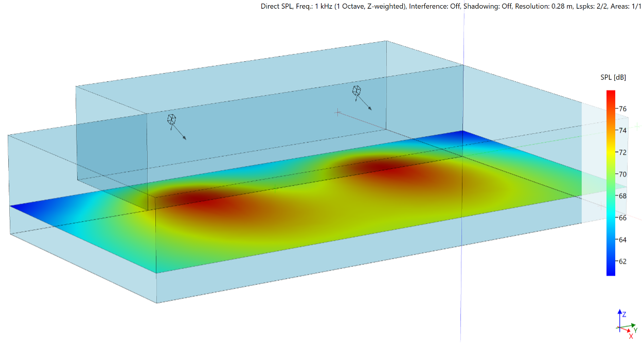
Figure 2 – Direct field coverage (1 kHz oct) with interference switched “off.” This shows a power summation of the two sources with no interference (power doesn’t cancel). The level delta over audience area has been reduced from 15 dB to about 6 dB.
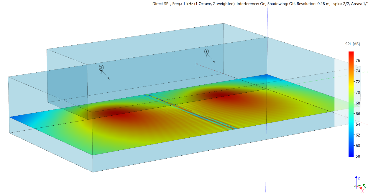
Figure 3 – Direct field coverage (1 kHz oct) with interference switched “on.” This shows the sound pressure summation of the two sources (pressure does cancel). The audience plane is mostly free of interference.
How About an Array?
Some might suggest that the loudspeakers be centrally arrayed. Figure 4 shows the 1 kHz octave band coverage with the loudspeakers separated by about 1 m, without changing the aiming. Figure 5 shows the loudspeakers aimed at +/- 30 deg.
Regarding an array:
1. When placed in close proximity the loudspeakers form a new single source with massive interference.
2. The interaction produces uneven coverage, as well as a “hot spot” below the array where a lectern is usually placed.
3. These loudspeakers lack sufficient pattern control to minimize their interaction. This is why re-aiming the loudspeakers had minimal effect on mitigating the interaction.
4. The coverage from this array is worse than the original system, with a new level delta of about 25 dB.
No amount of equalization, delay, or tuning can mitigate the problems caused by a poor array design. While aesthetically pleasing, the time and money spent will result in worse sound.
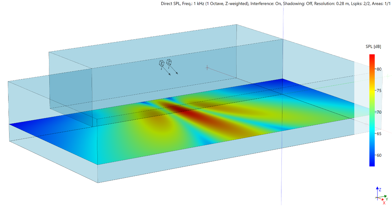
Figure 4 – The loudspeakers re-positioned to form an array. The coverage uniformity is destroyed.
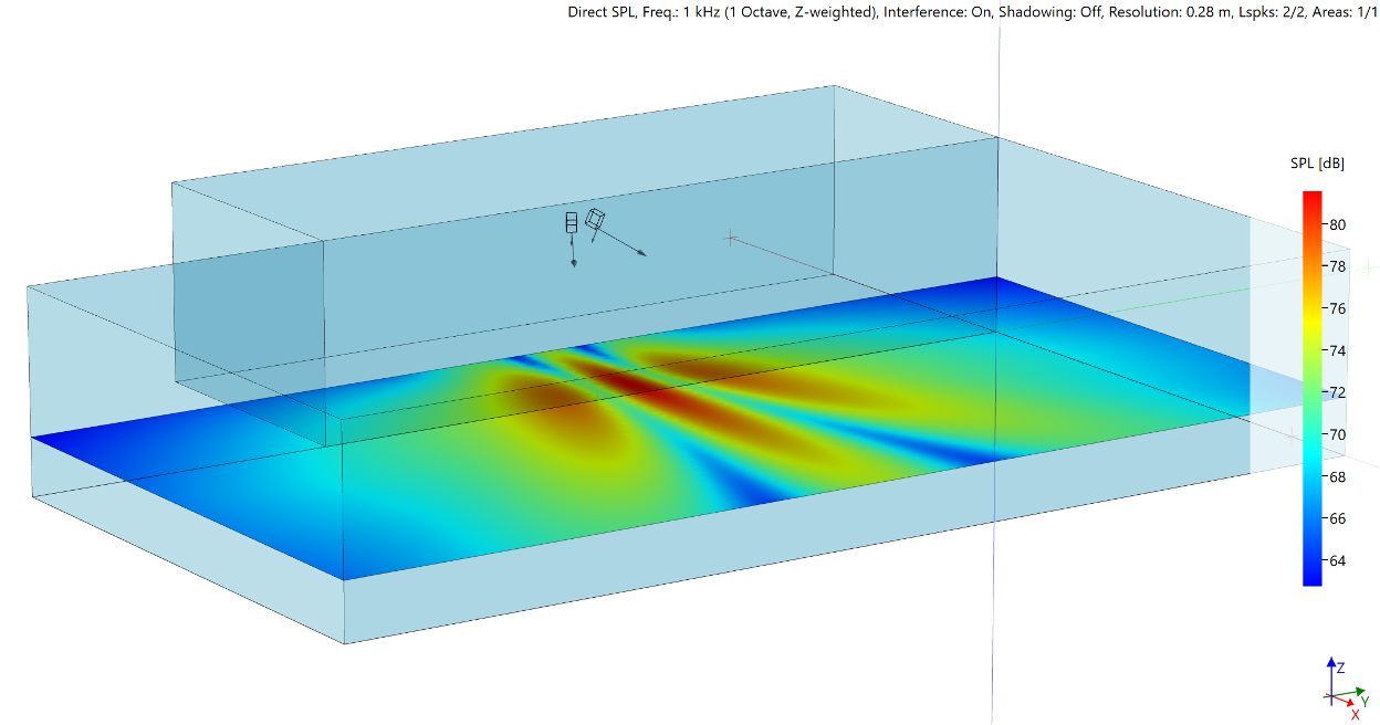
Figure 5 – The loudspeakers re-aimed to spread the coverage. Note that it is relatively unchanged. The source spacing determines the interference pattern. Increasing the source directivity can reduce the dB differential between lobes and nulls.
Frequency-Dependence
Coverage should always be considered at 1/1-octave resolution or higher. Figures 6 and 7 show all the octave bands of interest. The most important bands for music clarity and speech intelligibility are 1 kHz – 4 kHz.
Conclusion
The new zoned-distributed system has been used for several events. The venue owner reports vastly improved sound system performance.
“You can understand every word.”
“It no longer matters where you sit.”
“We never have feedback.”
The “fix” was loudspeaker placement. The objective for a sound system design is to achieve the best possible performance given the available resources. This venue is on a tight budget, and one simple design change dramatically-improved the system’s performance. The use of a computer model answered some fundamental questions that could be missed by intuition alone. pb
Zoned-Distributed Layout
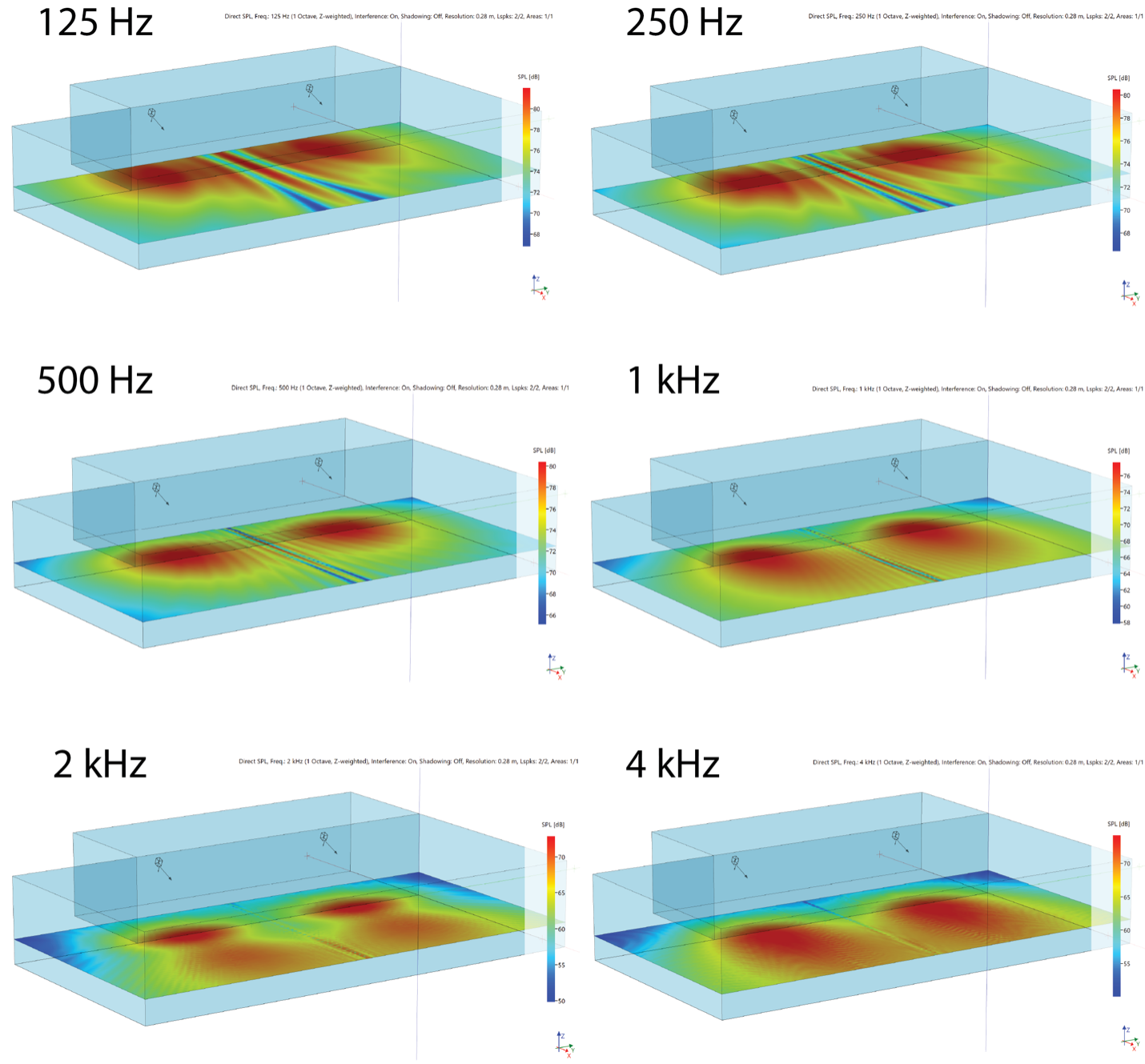
Figure 6 – Coverage maps of the zoned system for 1/1-oct bands. Note that the 2 kHz map shows the loudspeaker behavior in the crossover region.
Central Array
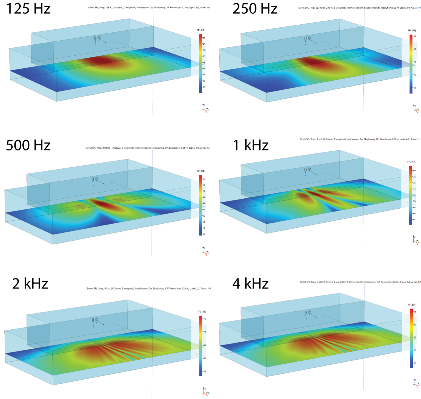
Figure 7 – Coverage maps of the array for 1/1-octave bands.
EASE 5® is a registered trademark of Ahnert Feistel Media Group (AFMG Technologies GmbH)