
Sample Rate Trade-offs
“Will my PA system sound cleaner if I run my mixer at a 96 kHz sample rate instead of 48 kHz?” The surprising answer is “No.”
Note: Grammatical errors in this article are proof that it was human-generated.
There. I’ve done it. I have challenged one of the Holy Grail tenets of digital audio and may have alienated a large contingent of the audio community. Before convicting me of Irrelevance, to await banishment to the Isle of Obsolescence please hear me out.
“More is better” – right? While there are times when that is true, it isn’t always the case in audio. A good example is the sample rate (SR) in an analog-to-digital converter (ADC). All digital products with analog inputs and outputs (I/O) have them.
It has not been long since the use of a 48 kHz SR was barely possible due to limits on processing power, data transport, storage, etc. Today’s ADCs can sample at many MHz (millions of hertz) and then decimate the SR to a practical value.
It is commonly believed that increasing the SR has the same effect on the audio signal as a higher pixel count in a digital camera. In the latter, the entire image is viewed in greater detail. Does a higher SR in a digital audio product (e.g 96 kHz vs. 48 kHz) capture the instruments and voices in greater detail, resulting in higher fidelity playback? Many claim to hear it. But is it true or is it the placebo effect?
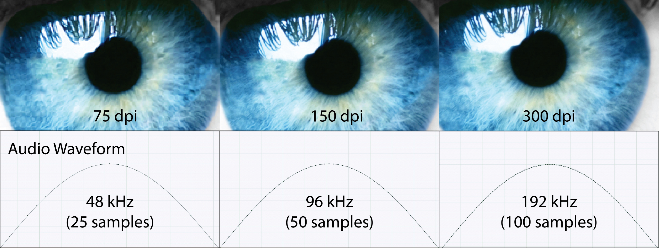 Figure 1 – Top: A digital photo at 3 resolutions (dots-per-inch). More pixels yield higher resolution. Bottom: One-half cycle of a 1 kHz sine wave, sampled at 3 different SR. The tiny dots are the samples. (Click to enlarge).
Nyquist-Shannon Sampling Theorem
According to the Nyquist-Shannon sampling theorem, the required sample rate to fully resolve an audio waveform must be slightly higher than two times the highest frequency that it contains. If we accept that the high frequency limit of human hearing is about 20 kHz, the required sample rate is slightly higher than 40 kHz. This justifies the default sample rate of 48 kHz for many digital audio devices. One-half the SR is called the Nyquist frequency, and it represents the approximate high frequency limit of the device. Figure 2 shows the choices of SR (and resultant Nyquist frequency) for a hypothetical digital mixer.
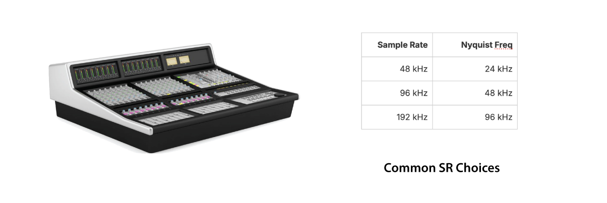 Figure 2 – For some digital audio products, the SR can be selected by the user.
So, selecting the SR sets the Nyquist frequency, which represents the upper limit of the devices frequency response. I produced a summary graphic to serve as a reference (Figure 3). There’s a lot there, so study it carefully. It shows the border between the analog and digital domains as determined by the SR. The ultimate objective is the production of high fidelity analog audio (the green-ish region) using digital audio technology (the red-ish region).
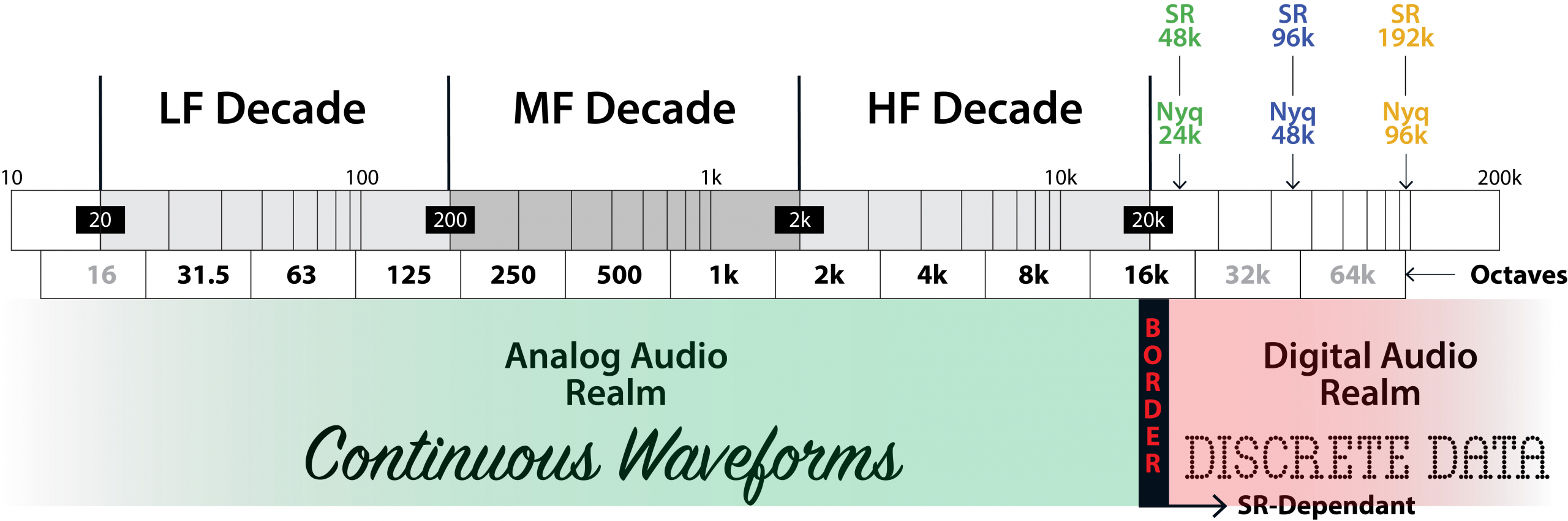 Figure 3 – The frequency spectrum of interest when considering the effect of the sample rate on the audio signal.
Trouble at the Border
From Figure 3, the sample rate determines the Nyquist frequency, which determines the upper limit of the device’s audio bandwidth. Doubling the SR doubles the Nyquist frequency. A 48 kHz SR extends the analog audio bandwidth to nearly 24 kHz. In musical terms, this captures all of the 16 kHz 1/1-octave band. A simple conclusion is that each SR doubling adds an additional octave of audio bandwidth.
This “bandwidth extension” is the main benefit from increasing the SR. A pure tone (sine wave) between 20 Hz and 20 kHz does not benefit from a higher-than-48 kHz sample rate. For that reason you don’t get a “tighter” kick drum from a higher SR unless the kick drum has harmonics that extend beyond 20 kHz. Even then, the playback system must be capable of reproducing the harmonics at the listener, who could be tens or hundreds of feet from the loudspeaker.
I performed some measurements on a digital signal processor (DSP) to demonstrate the effect that SR selection has on the HF limit. Figure 4 shows the overlaid frequency response magnitudes for three common SR. The impulse response (IR) for each is inset.
It is an unfortunate reality that steep cutoff filters producing ringing in both the time and frequency domains (also Figure 4). This has always been true, but is now more common due to the availability of “brick wall” audio filters. The ringing can be reduced by special processing techniques, but it is always present to some degree. It is not necessarily a byproduct of inferior parts or design.
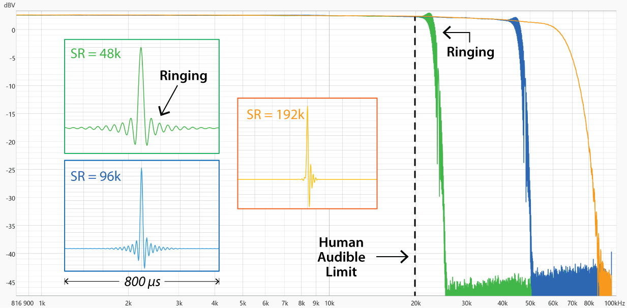 Figure 4 – The overlaid frequency response magnitude from 1 kHz – 100 kHz of three sample rates for a popular DSP. The IR for each is inset. The time span (800 μs) is the same for each IR.
-
Ringing can be reduced by increasing the SR.
-
The ringing for all three SR fall outside of the audible frequency range for humans (the vertical dashed line).
-
The frequency response to the left of the dashed line is identical for all three SR.
So, while ringing make look terrifying in a measurement, it is not likely to be audible.
Figure 5 shows the transfer function (TF) using 1/24-oct smoothing. The ringing artifacts are now invisible. Human hearing provides much greater smoothing, so not only are the ringing artifacts invisible, they are inaudible. There is a difference between what we can measure and what we can hear.
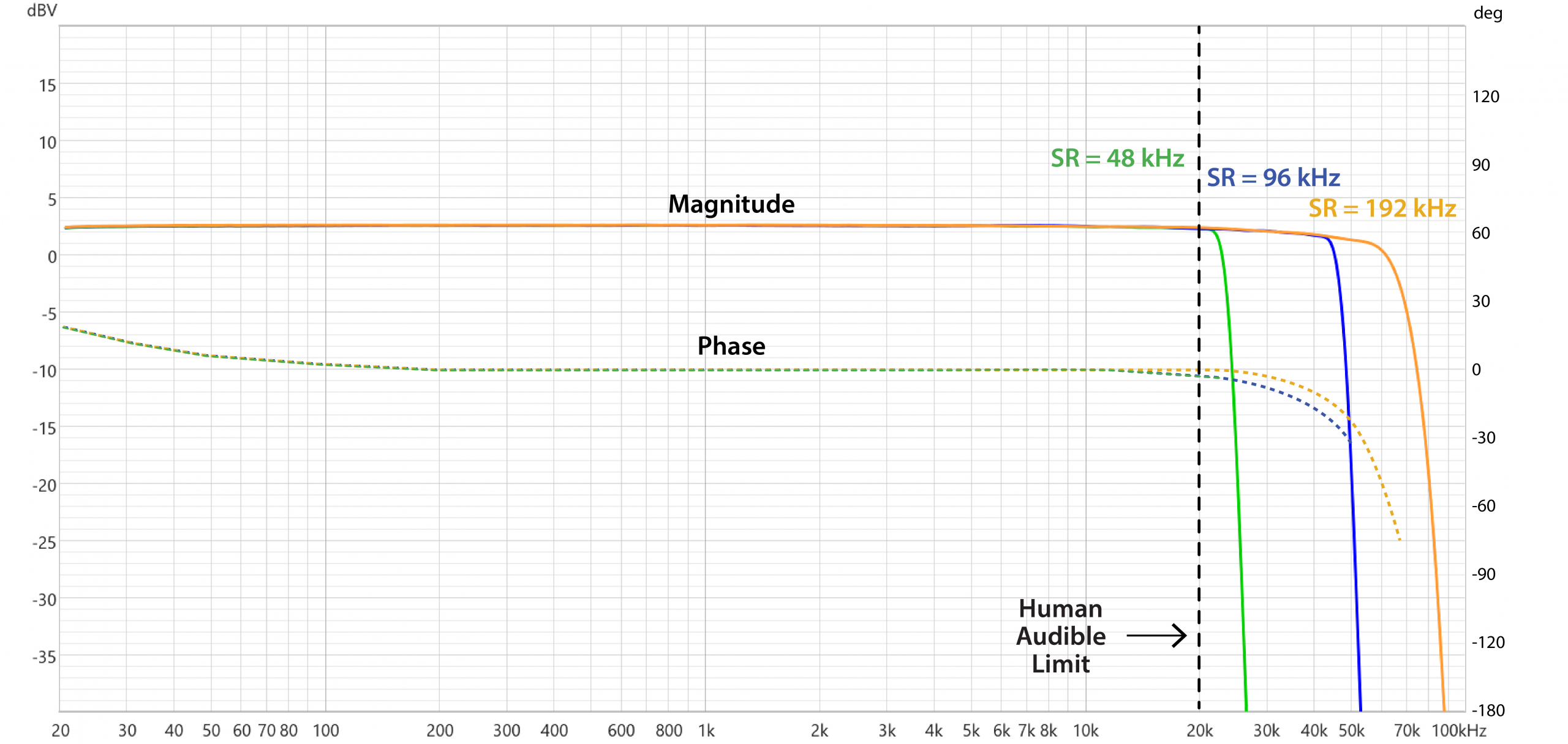 Figure 5 – The transfer function of the DSP using 3 sample rates. The plots are smoothed at 1/24-oct. All three are “flat” magnitude and linear phase through the human hearing range.
Why Use a Higher SR?
From the measurements it might seem that we should always use a 192 kHz SR. It produces the widest audio bandwidth and the least ringing. Here are some additional “pros” for increasing the SR beyond 48 kHz.
1. Reduced aliasing in digital processing
2. Gentler anti-aliasing and reconstruction filters (lower slopes reduce ringing)
3. Lower latency (in some systems)
There are other benefits, mainly relevant to heavy plugin processing used in studios and post production.
Why NOT Use a Higher SR?
As is always true in engineering, we never get something for nothing. Here are some “cons” for increasing the SR beyond 48 kHz.
1. Doubling the SR doubles the file size (for recording) and the required digital bandwidth for transporting the data.
2. A higher SR increases the CPU/DSP load. It can make fans run at high speed.
3. Increasing the analog bandwidth can allow the pickup and amplification of spurious interference signals produced by non-audio equipment (e.g. lighting).
4. Increasing the bandwidth increases the noise floor (Figure 6).
5. To realize potentially audible benefits, the higher SR must be maintained through the entire signal chain. This limits equipment choices and increases the system cost.
6. Sound reinforcement loudspeakers rarely have meaningful output beyond 20 kHz. They are engineered for high sensitivity and pattern control, not extended bandwidth.
7. Increasing the SR may decrease the maximum number of audio channels, especially for networked audio.
8. Some digital mixers and DSPs advertise a 96 kHz SR, but that is only for the internal processing. The actual SR is 48 kHz. There is no audio bandwidth increase due to the higher SR, so save your money on bumping up the other components to 96 kHz.
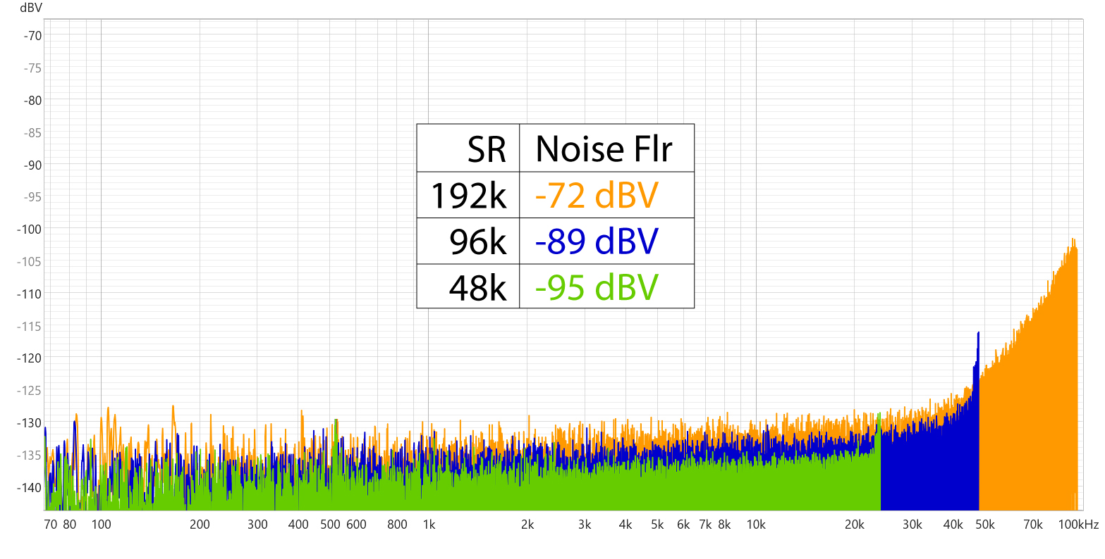 Figure 6 – The noise floor level increases with the SR. The difference is measurable, but not likely audible in a system with an optimized gain structure. Note: the noise floor level is found by summing the frequency bins.
FIR Filter Resolution
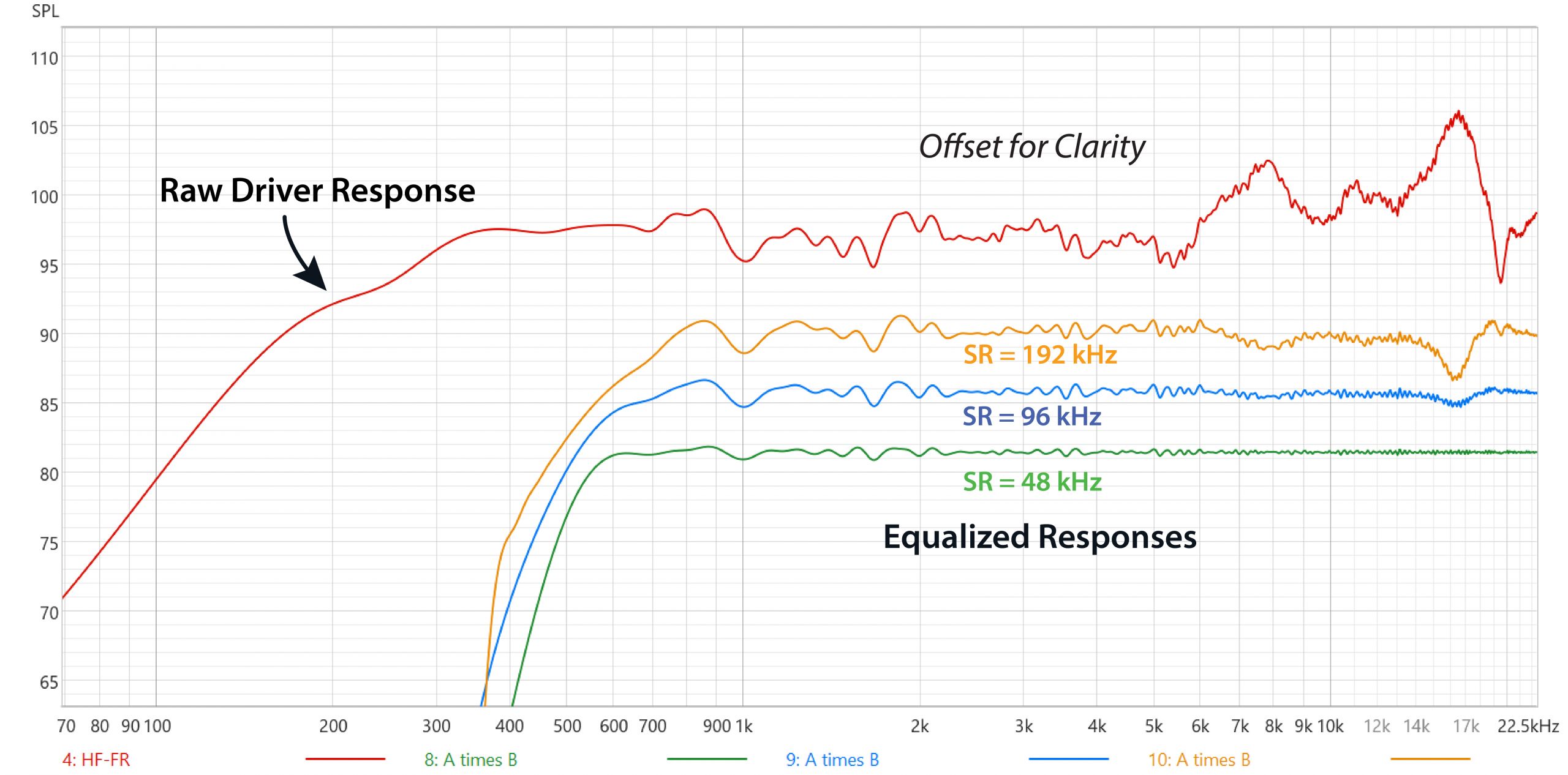
Perhaps the biggest drawback to increasing the SR is the reduction of FIR filter resolution. Doubling the SR halves the frequency resolution. This affects the filter detail as well as the usable low frequency limit. To demonstrate I measured a HF transducer and generated a corrective FIR filter (1024 taps). I also added a brick wall high pass filter at 500 Hz. Figure 7 shows the response at three sample rates. Note that the filter has more detail (increased frequency resolution) at the lowest SR (48 kHz). Figure 8 shows the frequency response magnitude of a loudspeaker for each SR. The lowest SR produces the smoothest response.
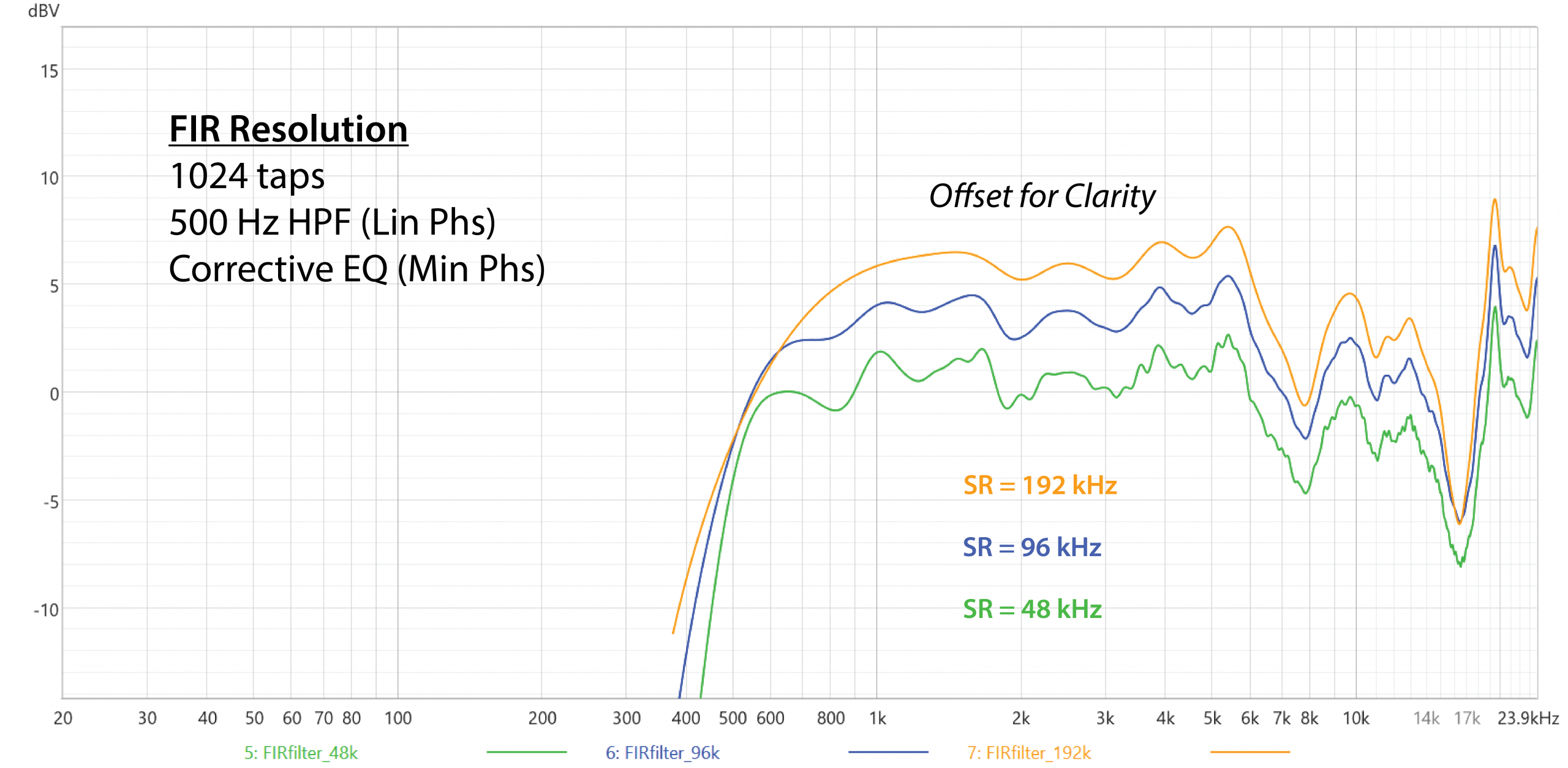 Figure 7 – Frequency response magnitude of a 1024 tap FIR filter for three sample rates. Note that the filter detail is higher using a 48 kHz SR.
The Reconstruction Filter
In a digital audio product the digital-to-analog converter (DAC) includes a reconstruction filter. It is a low pass filter that produces a continuous analog waveform from the samples. This is why a sine wave sampled at 192 kHz is not more resolute than one sampled at 48 kHz. The frequency response below the Nyquist frequency is identical for sample rates of 48 kHz, 96 kHz, and 192 kHz. This is true for any frequency up to the Nyquist frequency. The tangible benefit of the higher SR is the additional octave of analog bandwidth for each SR doubling. Returning to Figure 3, all three SR produce the same continuous analog waveform (the line beneath the samples).
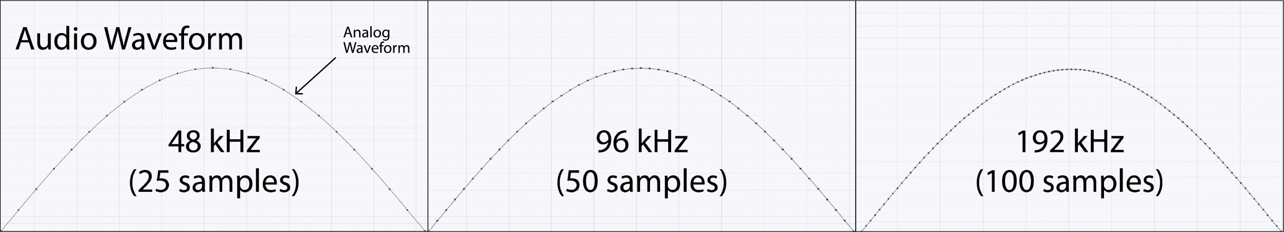
Figure 9 – The resolution of the 1 kHz sine wave does not increase with the SR. This is due to the reconstruction filter in the DAC.
In contrast, a digital photo (Figure 1) is a quantized version of the actual image. Increasing the dots-per-inch produces a higher resolution image. This is where the analogy between digital audio and digital imagery falls apart.
Summary
A SR that considers the bandwidth of human hearing must be selected. Good engineering practice suggests the use of the lowest appropriate SR. 48 kHz is a logical choice, which is why it is the default for many digital audio products. If you are considering using a higher SR, here are some things to keep in mind.
1. To realize the extra audio bandwidth the system response must increase one octave for every SR doubling. Microphones and loudspeakers pose the greatest challenge.
2. To realize the extended audio bandwidth the listener must be close enough to the loudspeaker to mitigate the high frequency loss due to air absorption. This suggests that near-field playback systems (e.g. studio monitors) and headphones give the greatest possibility of audio benefits from a higher-than-48 kHz SR.
Doubling the SR (and resultant system bandwidth) is expensive. Make sure that you understand why you are doing it, and that the results justify the extra processing load, data transport requirements, and extra expense. pb