Why 8 Ohms? – Part 2 – Voltage-Referenced Specifications
Despite their name, audio power amplifiers don’t amplify power. They produce a higher voltage copy of the input voltage, along with current as demanded by the load impedance.
As audio becomes increasingly digital, there remains two major design decisions rooted in analog technology. These are amplifier and loudspeaker selection.
In Why 8 Ohms? – Part 1 I showed why a loudspeaker impedance of 8 ohms became popular in the audio industry. It was logical. Sound systems were well-described by the voltage, current, and impedance magnitudes used for residential power distribution. (Figure 1). While there were certainly other motivations, practicable cable length and wire gauge considerations were instrumental in developing contemporary audio practices.
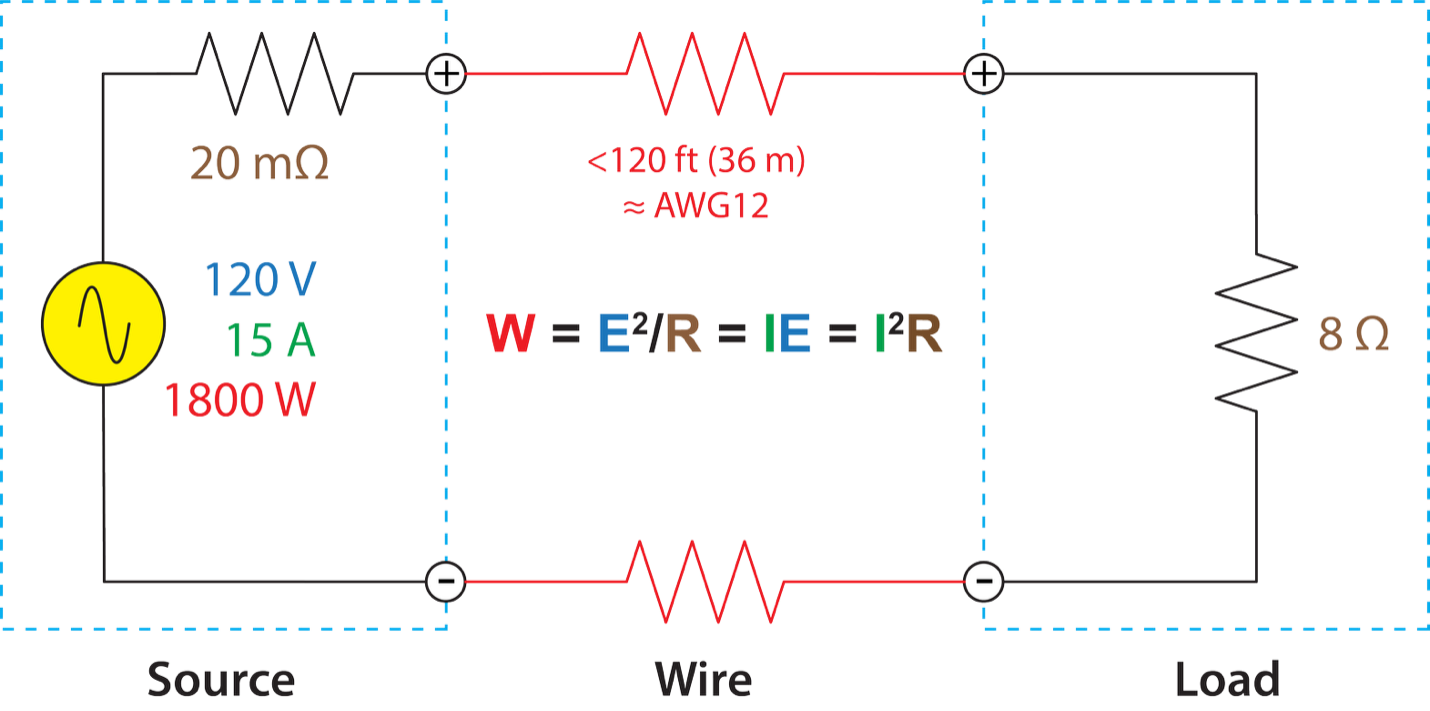 Figure 1 – An audio amplifier circuit is similar in scale to a utility power distribution circuit. W is power in watts, E is electro-motive force in volts, I is current in amps, and R is impedance in ohms.
The power mindset in audio came from utility power distribution. However, the dissimilarities between utility power systems and sound systems necessitate that audio power be separated into voltage, current, and impedance for deeper analysis.
Bill Whitlock summed it up nicely on the SynAudCon User Forum.
I think it might be important to point out that the term “power” is used rather loosely in speaker sensitivity testing. Since speaker impedances are well-known to vary substantially with frequency, it’s better to think in terms of VOLTAGE rather than power to avoid the tedious task of adjusting generator levels every time frequency is changed. Since 2.83 Vrms produces 1 watt in an 8 Ω resistor (the NOMINAL impedance of the speaker), the procedure is IMHO a fair way to measure sensitivity. – Bill Whitlock
To summarize, for practical reasons loudspeaker sensitivity must be measured with a standardized voltage rather than wattage. This is because the frequency response of a loudspeaker is voltage-dependent, not power dependent.
Amplifiers are Voltage Output Devices
Bill continues…
Bear in mind that audio power amplifiers are VOLTAGE output devices. Therefore, the actual power consumed in the speaker is highly variable with frequency. So, putting a flat frequency sweep through an amplifier does NOT produce a constant power in the speaker. Think of the 1 W as “nominal” power (a named quantity) – it assumes the speaker’s impedance is 8 Ω at any given frequency. Of course, this will make 4 Ω speakers show higher sensitivity, but we know to expect that. It’s part of the tradition. – Bill Whitlock
It’s also countered by the fact that a 4 Ω loudspeaker will have a lower maximum RMS voltage rating than an otherwise equivalent 8 Ω loudspeaker. There’s no 4 Ω advantage when you take the maximum SPL into account.
His statement regarding audio power amplifiers is important. A “voltage output device” is optimized for voltage-transfer, where the output voltage is independent of the load impedance. This is the constant voltage (CV) interface.
Here’s how it works. A signal voltage is applied to the amplifier’s input. It is increased by the amplifiers gain to produce the amplifier’s output voltage. This voltage is applied to the load (a loudspeaker or resistor) and current flows through the load. The amplifier’s output voltage and available current are determined by the amplifier’s design team and must be appropriate for the amplifier’s intended application. The amplifier’s voltage is measured across a test resistor to rate the amplifier in watts. Power ratings come from voltage measurements.
While audio power remains a quantity-of-interest when deploying amplifiers and loudspeakers, the voltage is what is measured to rate the amplifier and characterize it regarding level, distortion, and fidelity.
Load Impedance
The need for a CV interface becomes obvious when we consider the load that the amplifier must drive – a loudspeaker. As Bill pointed out, the loudspeaker’s impedance can vary wildly with frequency (Figure 2). We need for this to not matter, and it doesn’t in a CV interface. If a sine wave sweep is applied to this load from a constant voltage source, it will produce the same voltage at every frequency (Figure 3).
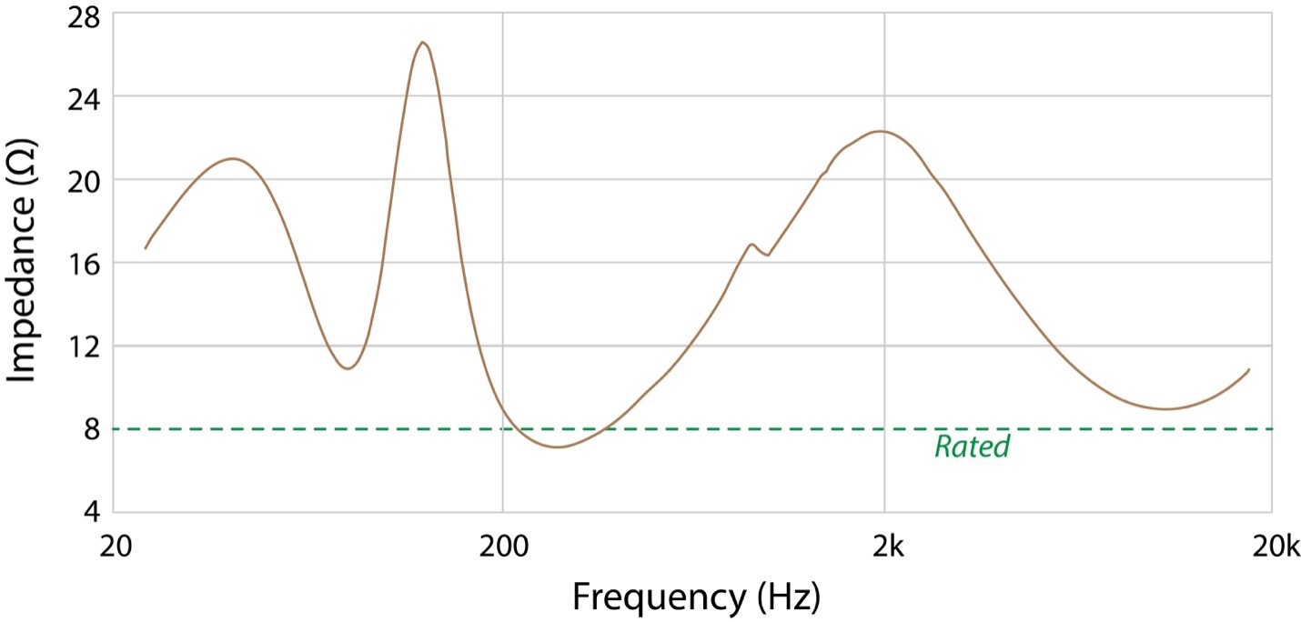 Figure 2 – The impedance magnitude of a multiway, passive loudspeaker.
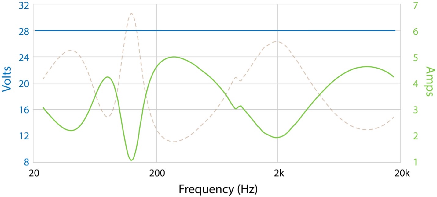
Figure 3 – The amplifier-to-loudspeaker current flow (green) that results from a swept sine wave (blue). The current (and power) are frequency dependent. The voltage (of this signal) is the same at every frequency.
The Theoretical Roots
Figure 4 shows a hypothetical amplifier with infinite available current. Idealized reference cases like this one are useful for conveying concepts. The impedance used for amplifier testing is a test resistor.
Note that the output voltage (column 1) is independent of the load impedance (column 3). The voltage is unaffected as the load impedance is reduced. The current draw (column 2) increases with decreasing load impedance, but the voltage stays rock solid. Of course, during actual use the voltage will be an audio signal. It may be a tone, noise, music, or speech, but the waveform shape and magnitude are unaffected by the loudspeaker’s impedance.
Don’t confuse this with the use of the term to describe transformer-distributed loudspeaker systems. Nearly all amplifier-to-loudspeaker interfaces are constant voltage, with or without distribution transformers. The take-away is this. The output voltage of an audio amplifier should not be affected by the load impedance. One needs only to track the voltage to design and troubleshoot sound systems. If the impedance is known, the current and power can be calculated (if needed) using the measured voltage and the power equations (Figure 1).
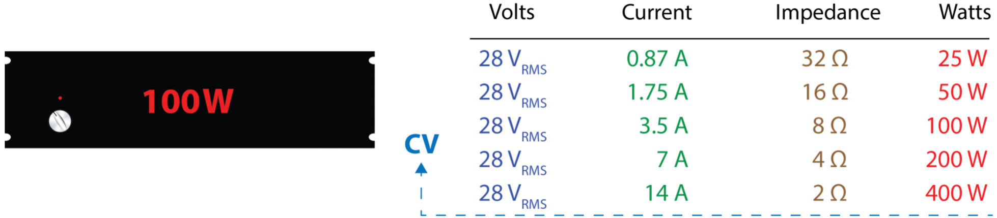
Figure 4 – Amplifier A. This is an idealized amplifier with infinite available current. It is constant voltage for any load value. Its power rating (100 W) is for an 8 ohm load.
Now that I have presented an idealized example, let’s look at a real-world amplifier (Figure 5). This amplifier is constant voltage, but only down to the amplifier’s minimum rated load impedance. Why not lower? Current is expensive. Increasing the available current increases the price of the amplifier. For this reason, a manufacturer may only guarantee CV behavior down to a minimum impedance (usually 8, 4, and sometimes 2 ohms) and with high crest factor signals (e.g. speech and music). This allows them to value engineer the amplifier by not supporting extremely low load impedances and/or low crest factor signals (e.g. sine waves).
By using voltage-referenced ratings we are not abandoning power ratings. They have their place. It’s just that given the use of the CV interface, the voltage is the quantity of interest. Since manufacturers rate the amplifier in watts, not volts, you can calculate the maximum output voltage from the 8 Ω power rating (Figures 8 and 10).
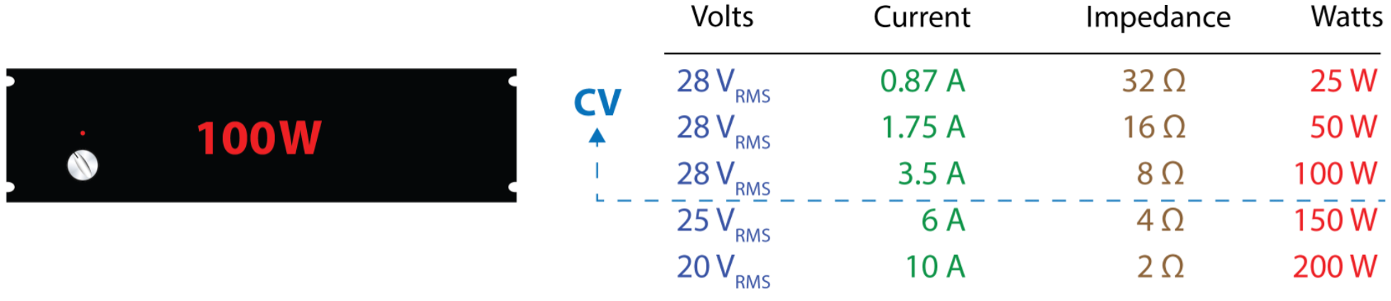
Figure 5 – Amplifier B. This is real-world amplifier with finite available current. The loads for which it is constant voltage are indicated. Its power rating is for an 8 Ω load.
Voltage Linearity vs. Load Impedance
The maximum linear output level of an amplifier is limited by an acceptable distortion level, such as 1% Total Harmonic Distortion (THD). An additional criterion is the voltage linearity vs. load resistance. To faithfully reproduce the applied audio waveform, the amplifier’s output voltage must be independent of the load impedance. If it changes with load impedance, so does the audio signal and the resultant sound. The fidelity is reduced.
The Common Amplifier Format (CAF) used in SynAudCon training courses measures the amplifier’s voltage and current at 1x, 2x, and 4x its minimum rated load impedance using three signal types (sine burst, sine continuous, and noise). The amplifier’s rated output voltage and power can be determined from the resultant data matrix (Figure 6). Note that 8 ohms is the lowest resistance for voltage linearity in this example. For this reason, nearly all audio amplifiers have an 8 Ω power rating. I’ll come back to that.
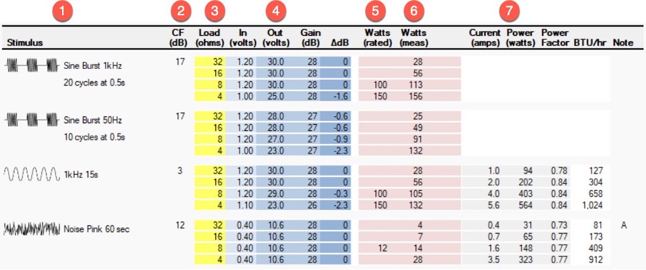
1. Stimulus type
2. Stimulus crest factor
3. Load resistance
4. IO voltage and gain
5. Rated power
6. Measured power
7. AC power draw (for sizing AC power circuit breakers)
Figure 6 – The CAF presents the amplifier’s output voltage for multiple load resistances. The amplifier’s power rating (column 5) can be determined from this matrix.
CAFViewer™ – A More Complete View of Amplifier Performance
Can a one number power rating characterize an amplifier? Of course it can’t. Our freeware viewer/calculator gives a bigger picture. CAFViewer™ (https://caf.prosoundtraining.com) loads with an example report containing multiple amplifier tabs (Figure 7). These are actual amplifiers that have been genericized for inclusion with the viewer. Use this resource to train your amplifier intuition by studying the tabs. Each data matrix reveals how the amplifier received its rating.
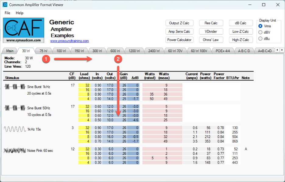
Figure 7 – In CAFViewer, toggle through the amplifier tabs (1) and observe the amplifier’s voltage vs. load (2) for the sine burst 1 kHz, sine burst 50 Hz, and continuous sine 1kHz. Note how the rated power is determined.
Loudspeaker Sensitivity
The sensitivity of a loudspeaker can be measured at any voltage and there are an infinite number of possibilities. We need to choose one. There is utility in using a voltage that is tied to legacy sensitivity specifications. Sensitivity has traditionally been referenced to “1 W.” This makes the voltage component for an 8 ohm loudspeaker 2.83 Vrms (+9 dBV). The relationship is shown in Figure 8. By using 2.83 Vrms, existing “1 W” sensitivity ratings become numerically the same as voltage-referenced sensitivities using 2.83 Vrms.
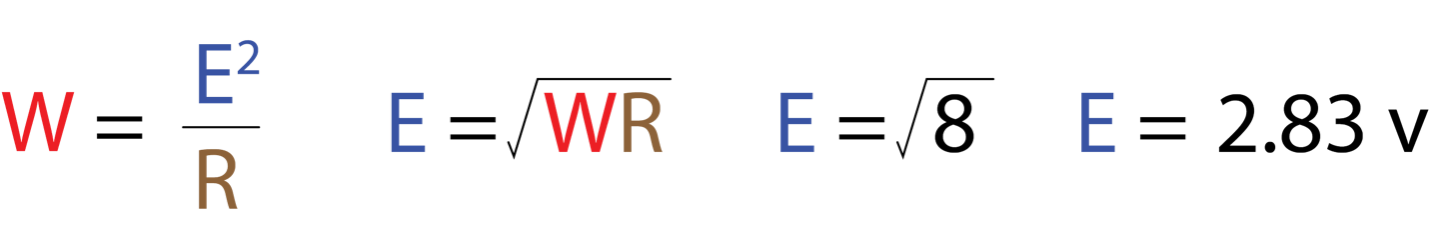
Figure 8 – A loudspeaker’s sensitivity, formerly referenced to 1 W, 8 ohms is now referenced to 2.83 Vrms.
The 8 Ω Portal
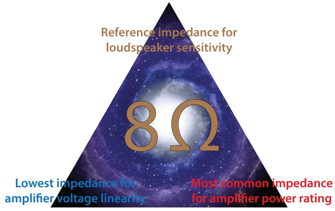
Let’s consider the significance of 8 ohms. It is common denominator between several aspects of audio systems. It is
– The reference impedance for loudspeaker sensitivity
– The lowest impedance at which most amplifiers exhibit voltage linearity
– The most common impedance for amplifier and loudspeaker power ratings
8 ohms serves as a portal for transitioning from power ratings to voltage ratings.
These examples show the sound level produced by a “100 W” amplifier connected to a loudspeaker using both power and voltage. Voltage-based calculations are independent of impedance and allow troubleshooting with only a voltmeter.
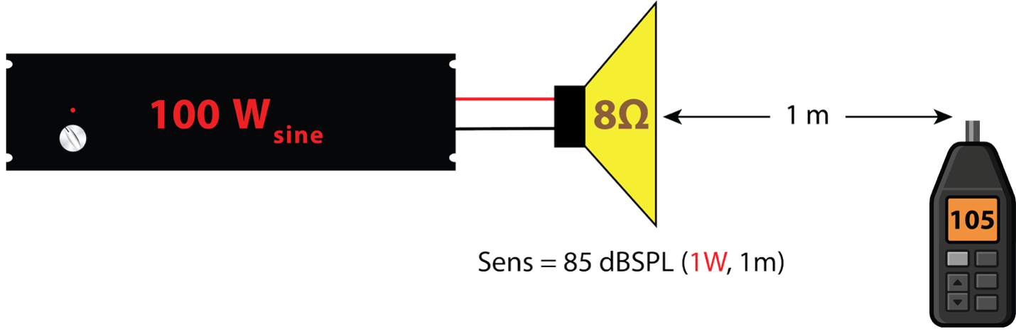
Figure 9 – The traditional method of amplifier rated in watts, and loudspeaker sensitivity referenced to 1 W
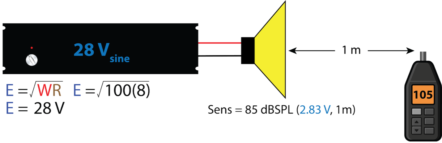
Figure 10 – Same as Figure 9, using only voltage. Note that the resultant sound level (105 dB) is the same as for the power-based example. The load impedance is not needed.
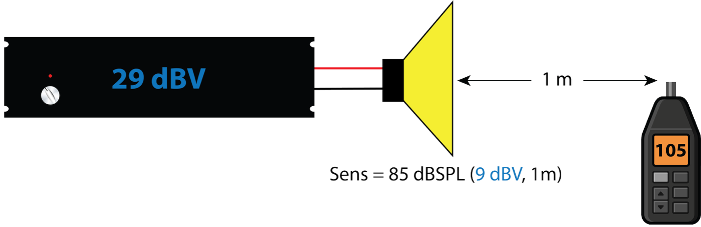
Figure 11 – Same as Figure 10, using level (dBV) instead of volts.
To summarize, voltage-referenced ratings produce the same result as power-referenced ratings and have the advantage of being independent of impedance and easier to measure.
Internally Powered Loudspeakers
While it may initially seem illogical and confusing, the sensitivity of an internally powered (or active) loudspeaker can also be referenced to 2.83 Vrms. The active loudspeaker is treated like a “black box” with 2.8 Vrms applied to the input. The 1 m SPL is measured to determine the system sensitivity (Figure 12).
In this case, the sensitivity also includes the amplifier’s gain. The result is a very high sensitivity rating since most amplifiers have 26 – 32 dB of gain. In practice, +9 dBV into a line level input (the loudspeaker) will be really loud. A lower drive voltage can (and should) be used, with a correction factor to normalize it to 2.83 V (9 dBV).
Using this method the actual amplifier gain, and transducer sensitivity are not known, but it doesn’t matter. The resultant sensitivity is correct. Unlike passive loudspeaker sensitivities, the sensitivity of an active loudspeaker will be very near its maximum SPL.
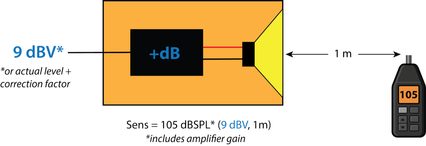
Figure 12 – The sensitivity of active loudspeakers can also be referenced to 2.83 Vrms. This reveals the combined response of the amplifier and loudspeaker. Note that the resultant sound level (105 dB) is the same as the passive loudspeaker examples.
Maximum Input Voltage and Maximum RMS SPL
Knowing the loudspeaker’s sensitivity is a means to an end. Once connected to an amplifier, the pair will produce a sound pressure level at the listener. Whether it’s a low sensitivity loudspeaker paired with a large amplifier, or a high sensitivity loudspeaker paired with a small amplifier, the result is a maximum linear sound level at a reference position. My examples use a sine wave, but in practice the signal will usually be shaped pink noise. Noise has a higher crest factor (lower RMS voltage) than a sine wave.
Using 2.83 Vrms to measure the loudspeaker’s sensitivity, and knowing the output voltage of the amplifier, we can exactly calculate the sound level at a listener using only voltage for “Low-Z” loudspeaker systems. “High-Z” distribution systems, such as 70.7/100 V transformer distribution systems still use power taps to determine the load placed on the source. CAFViewer handles both system types (Figure 7). The launch button for each calculator is at the top-right of the CAFViewer home screen.
From Then to Now
Nearly a half-century ago the audio industry moved away from power-referenced levels for the audio signal chain. The dBm (600 Ω) evolved into dBu (dB ref. 0.775 Vrms). The dBV (dB ref. 1 Vrms) was introduced as an optional reference. Both assume a CV interface. The use of voltage references for amplifiers and loudspeakers completes the transition (Figure 13). Whether the workflow is
Voltage → Power → Voltage
or just
Voltage
with the CV interface the result is exactly the same. Why go through the extra steps to express the voltage as power in watts?
If you practice audio, you’re in the voltage business. – pb
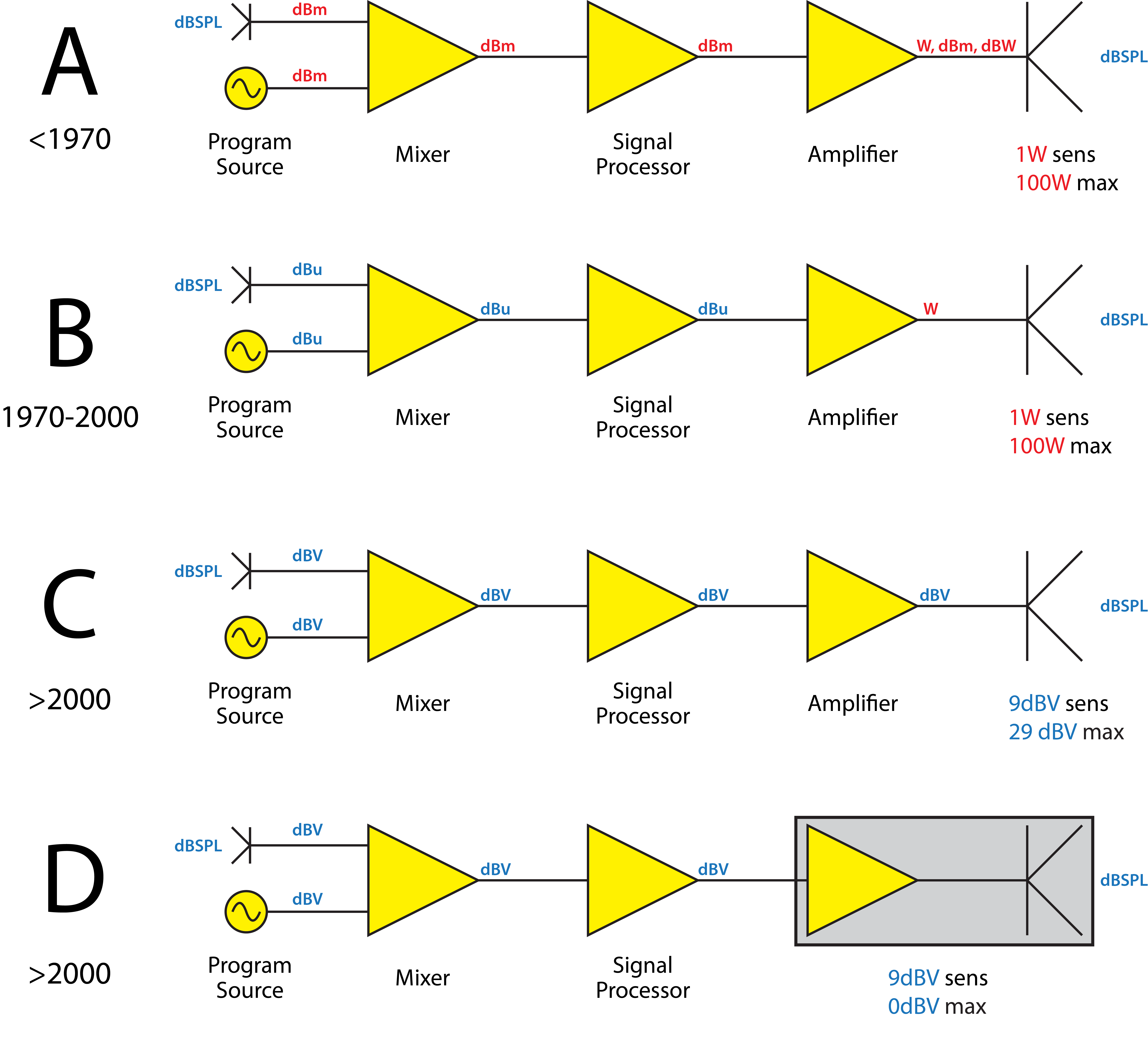
Figure 13 – Audio levels through the ages. A: Power ratings for all components. B: Voltage (or dBV, dBu) for all but amplifier/loudspeaker. C and D: Voltage (or dBV) for the entire signal chain. DBu can be used in lieu of dBV by adding 2.2 to the dBV level.